2014 Student Blog Post #4: John Arnold

My name is John Arnold and I’m a Ph.D. student in Michigan Tech’s Industrial Heritage and Archaeology program.  I’m an architect by training and until recently had been practicing in Washington state, before returning to school to study Historic Preservation at the University of Oregon, where I focused my studies on the 3D digital documentation of historic buildings.  I’ve been working closely with the mapping teams, which has been very interesting for me because of my familiarity with crafting scaled drawings both by hand and with digital visualization and data management tools—in a different field.  Mapping sites and landscapes as an archaeologist has been a fascinating complement to those practices.

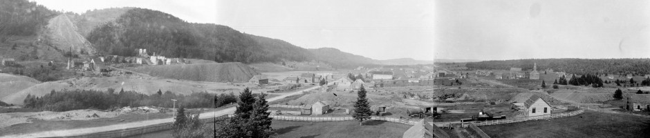
Author John Arnold working in the “interyard” area of Clifton.

Mapping the cemeteries, part 2

The other “pre-digital” method employed in this mapping project used an optical transit and stadia rod. It was a great experience for us as students to have the opportunity to use these traditional survey tools. These are entirely manual instruments and I enjoyed the feel of a little mystery while learning to use them. Their historic feel and mystery did not mean they were easy to use! In fact, I found using an optical transit had a fairly steep learning curve, and every student in field school got to work through it. The potential for error reinforces the importance of copious field notes and sketches made by every student in their field journal. Dr. Scarlett has blogged about this before.

The transit is set up on its tripod at a marked and knowable location, so that all measurements taken can be integrated into the network of points being recorded on the site map. An ideal position for the transit provides a clear line of sight to other known and recorded points, such as site boundary markers or significant site features, while simultaneously allowing for new, unknown points to be located. The challenges begin with the simple-sounding step of the level positioning the tripod at a comfortable eye height directly over a known control point. This might be easy enough on flat and level ground, but in the field, it is a real trick! However, getting this done correctly establishes a good foundation for the leveling of the transit head.

Team member Eric Pomber taking readings from the optical transit in the Catholic cemetery.

The transit head consists of a monocular scope that pivots in two dimensions (up-down and left-right rotation), both of which are calibrated by integrated protractor elements used to measure angles from an established zero point. The transit head, once mounted to the tripod, must be leveled using a series of set screws. The optical scope is secured at a horizontal level, such that turning it on its vertical axis sweeps a horizontal plane over the site. The height of the transit above grade is taken, as this will be needed later to calculate relative heights over the uneven terrain. In addition, a “zero” angle is established against which subsequent measured angles are set.

This is an optical transit, similar to the model used by Michigan Tech Industrial Archaeology students when they learn the basics of surveying and map making. Creative Commons image courtesy of Land Surveying Services, Inc.

The transit team consists of two or perhaps three members: one person hold the stadia rod at a previously-determined landscape feature (such as something noted and flagged during the pedestrian survey), while another reads the instrument, and, if they are lucky, a third person takes notes and double-checks the readings. The stadia rod is demarcated with centimeter and meter increments that are easily discernable through the scope — if, that is, there is a clear line of sight between the two. Often creating a clear line of sight in the conditions of a heavily overgrown site requires the third helper to hold brush aside while the readings are taken.

The optical scope has one vertical and three horizontal crosshairs within it; the scope is designed such that the vertical distance between the uppermost and lowermost crosshairs as measured against a distant stadia rod can be translated with a simple calculation to provide the distance from the transit to the stadia rod. The height of the top, middle, and low crosshairs are recorded as read from the stadia rod, and the angle measurement from zero is recorded from the transit head itself. With these measurements in hand, the location of the feature being sighted in can be plotted on the map.

This schematic diagram shows computations of distance using stadia measures, when the transit is level. Creative Commons image courtesy of the Food and Agriculture Organization of the United Nations.

This process is repeated for as many features as desired–and can be sighted–from the control point. As it so happens, in the wooded and hilly terrain of Hillside Cemetery requires additional control points to be established. As with locating the initial control point, a good location with visibility to several known features as well as many new, unmapped, features is selected; this new control point is “shot in,” or located, in the same way as other features. The transit and tripod are then carefully packed up and moved to the new control point-while it might be tempting to simply pick up and lug the instrument across uneven terrain to its new location, best practice dictates keeping good care of the sensitive and valued transit. At the new location, the transit head is set to level, as before, but now the first feature to be located is the last control point, calle “backsighting.” Doing so not only provides a second measurement of the distance between the two points, but allows the angle measurements from the first control point to be consistent with those from the second point.

As a simple example, if the second control point is established at a 90° angle from zero of the first control point, the back-sighted angle measurement will be 270°– the zero reading is translated from the first to the second control points, and all of the features being located can be measured against the same, shared zero. As an illustration, imagine yourself standing on a benchmark, facing north. If you point straight out to your left, without rotating your body, you will be pointing at 90° measured counterclockwise. Now move yourself 10 paces in that direction, and face north; your zero is the same, north, and if you point at where you had been standing, without rotating your body, you will be pointing straight out to your right, to 270°. Again, this requires a great deal more care under field conditions, but the principle is the same.

This procedure proved to be an enjoyable and fruitful process for everyone involved, and was used not only to locate distant points that could not be readily located with triangulation, but as a double check against other triangulated points. The process of directly engaging the world without digital intermediaries was a wonderful introduction to mapping techniques used in field archaeology.

Dan Schneider transfers carefully recorded data points to the scaled master drawing in the field.